Low-Density Parity Check Codes(LDPC): A crucial component of contemporary communication systems intended to improve data transmission reliability is Low-Density Parity-Check, or Low-Density Parity Check Codes, coding.
These codes ensure that the information received is as similar to the original message as feasible by identifying and fixing faults that happen when data is transmitted across noisy channels.
Because of their reliability and effectiveness, Low-Density Parity Check Codes codes are a vital component of many digital communication systems.
Both wireless and cable communication systems benefit from their usefulness in controlling mistakes and enhancing data integrity.
This blog gives an overview of Low-Density Parity-Check (LDPC) codes, covering topics such as their history, encoding and decoding procedures, and more.
Understanding of Low-Density Parity Check Codes
A linear error-correcting code called Low-Density Parity-check (LDPC) code is used to send messages over a noisy transmission channel.
An Low-Density Parity Check Codes is built on top of a sparse Tanner graph, which is a bipartite graph subclass.
Since LDPC codes are capacity-approaching codes, it is possible to set the noise threshold for a symmetric memoryless channel extremely near to its theoretical maximum, or the Shannon limit, by practical techniques.
The chance of lost information can be reduced to the appropriate level up to the upper bound set by the noise threshold for the channel noise.
Time linear in the block length can be achieved in the decoding of LDPC codes by the use of iterative belief propagation techniques.
The LDPC decoder is used for Forward Error Correction (FEC) in systems where transmitted data is subjected to errors before reception, e.g., communications systems, disk drives, and so on.
LDPC Codes are part of recently invented ‘Iterative decoders’, which involve multiple iterations to improve performance. Iterative decoder shows improved performance compared to legacy convolution codes.
LDPC codes outperform Convolution codes by 3-4 dB and are characterized by a ‘water-fall’ region in their SNR – BER curve.
There is an SNR threshold after which BER decreases very rapidly. Hence, LDPC codes have found their place in most of the latest standards including Wi-Fi (802.11n, 802.11ac), Wi-Max (802.16e), DVB-S2, and 3GPP-LTE Advanced.
History of LDPC
In honor of Robert G. Gallager, who created the LDPC concept in his PhD dissertation at the Massachusetts Institute of Technology in 1960, LDPC codes are also referred to as Gallager codes.
It wasn’t until 1996 that his work was uncovered that LDPC codes were remembered.
In the late 1990s, Turbo codes a different class of capacity-approaching codes that had been found in 1993 became the standard coding scheme for satellite communications and Deep Space Network applications.
Following that, LDPC codes attracted new attention as a patent-free substitute with comparable functionality.
Since then, low-density parity-check codes have improved to the point that they outperform turbo codes in the higher code rate range and error floor, making turbo codes more appropriate for lower code rates exclusively.
Block Code Basics/Operational Use
A sparse parity-check matrix defines the functional characteristics of LDPC codes. The sparsity restrictions governing the LDPC code creation are addressed subsequently.
Typically, this sparse matrix is produced at random. Robert Gallager created these codes for the first time in 1960.
A sample LDPC code utilizing Forney’s factor graph notation is shown in the graph fragment below.
This graph has (n−k) constraint nodes at the bottom and n variable nodes at the top connected.
This is a commonly used visual aid for a (n, k) LDPC code representation.
When the components of a valid message are arranged on the Ts at the top of the graph, the graphical requirements are satisfied.
In particular, every value connecting to a factor node (a box with a ‘+’ symbol) must add up to zero, modulo two (i.e., it must total up to an even number, or there must be an even number of odd values); all lines connected to a variable node (a box with a ‘=’ sign) have the same value.

Eight possible six-bit sequences match valid codewords, ignoring any lines that travel outside of the image: 000000, 011001, 110010, 101011, 111100, 100101, 001110, 010111.
A three-bit message encoded as six bits is represented by this snippet of LDPC code. Here, redundancy is employed to boost the likelihood of recovering from channel faults.
This code is linear (6, 3), where n = 6 and k = 3.
Once more disregarding lines that exit the image, the parity-check matrix that represents this section of the graph is

One of the three parity-check requirements is represented by each row in this matrix, and the six bits in the received codeword are represented by each column.
The eight codewords in this case can be obtained by inserting the parity-check matrix
H into this form 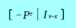 through basic row operations in GF(2):

Step 1: H.
Step 2: Row 1 is added to row 3.
Step 3: Rows 2 and 3 are swapped.
Step 4: Row 1 is added to row 3.
From this, the generator matrix G can be obtained as 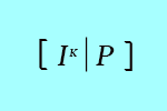 (noting that in the special case of this being a binary code
 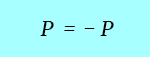 ), or specifically:

Finally, by multiplying all eight possible 3-bit strings by G, all eight valid codewords are obtained. For example, the codeword for the bit-string ‘101’ is obtained by:

where ![]() is a symbol of mod 2 multiplication.
is a symbol of mod 2 multiplication.
As a check, the row space of G is orthogonal to H such that GHT=0
The bit-string ‘101’ is found in as the first 3 bits of the codeword ‘101011’.
Encoding Process
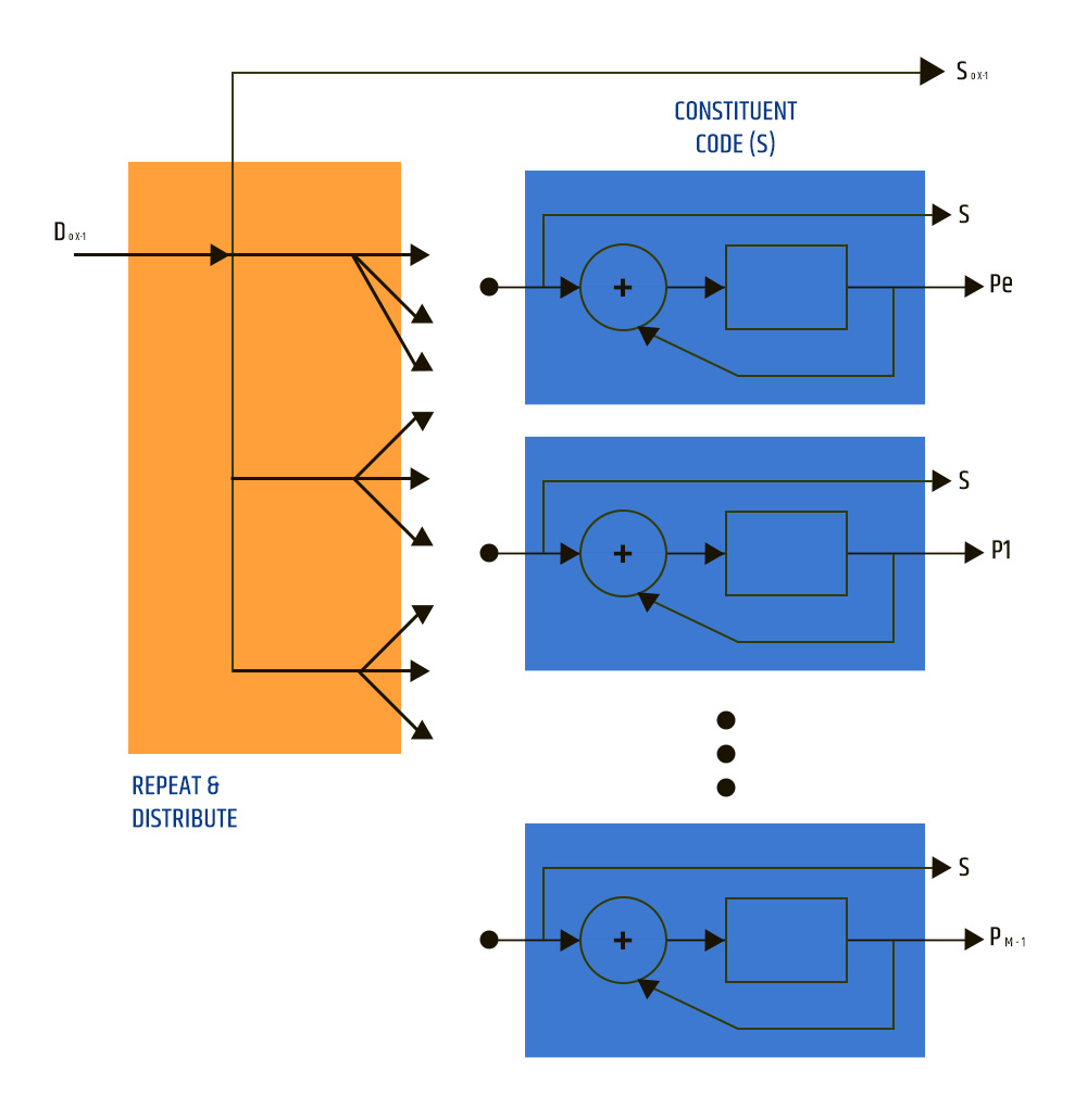
The input data bits (D) are repeated and sent to several constituent encoders during the encoding of a frame.
Usually, the constituent encoders are accumulators, and a parity symbol is produced by each accumulator.
To create the code symbols, a single copy of the original data (S0, K-1) is transferred along with the parity bits (P). Every constituent encoder’s S bits are thrown away.
Another constituent code may make use of the parity bit.
In an example, the encoded block size is 64800 symbols (N=64800) with 43200 data bits (K=43200) and 21600 parity bits (M=21600) using the DVB-S2 rate 2/3 code.
Except the first parity bit, which encodes 8 data bits, each constituent code (check node) encodes 16 data bits.
The remaining 4680 data bits are utilized in 3 parity codes (irregular LDPC code), while the first 4680 data bits are repeated 13 times and used in 13 parity codes.
In contrast, two constituent codes that are set up in parallel are usually used in conventional turbo codes, each of which encodes the whole input block (K) of data bits.
Recursive convolutional codes (RSC) of intermediate depth (eight or sixteen states) make up these constituent encoders. One copy of the frame is interleaved between each RSC by a code interleaved.
As opposed to this, the LDPC code employs numerous low-depth constituent codes (accumulators) simultaneously, each of which only encodes a tiny percentage of the input frame.
The many constituent codes can be understood as multiple low-depth (2-state) “convolutional codes” coupled by the distribution and repeat operations.
In the turbo code, the repeat and distribute operations serve as the interleaved.
More flexibility in the design of LDPC codes is provided by the ability to more precisely control the connections between the various constituent codes and the degree of redundancy for each input bit.
In some cases, this can result in higher performance than turbo codes. At low code rates, turbo codes still appear to outperform LDPCs; at the very least, turbo codes make it simpler to create low-rate codes that work well.
In practical terms, the accumulators’ hardware is utilized throughout the encoding procedure.
In other words, the same accumulator hardware is used to generate a new set of parity bits after the previous set is generated and the parity bits are saved.
LDPC Decoding Algorithm
The decoding algorithm for LDPC codes was found multiple times independently and goes by several names.
The belief propagation algorithm, the message-passing algorithm, and the sum-product algorithm are the most widely used ones.
The exchange of messages between the check and variable nodes is how the decoding algorithms function.
A value proportionate to the likelihood or “belief” in the “correctness” of the received bit is contained in these messages.
Node C0 transmits a message to F1 and F3 in the first step, and Node C1 sends a message to F0 and F1, and so on.
Every check node fj computes a response to each associated variable node in the second phase.
Assuming that the other v-nodes connected to fj are accurate, the response message contains the value that fj thinks is correct for this v-node, ci.
Put differently, each c-node (fj) in the example is connected to four v-nodes.
Therefore, a c-node fj determines the value that the fourth v-node needs to have in order to satisfy the parity-check equation after examining the message that it has received from three v-nodes.
The method ends at this point if all of the parity-check equations are satisfied.
If not, the v-nodes get the messages from the check nodes and utilize this extra data to determine whether the bit they initially received was acceptable. A majority vote is an easy approach to resolve this.
Bit flipping algorithm
Assume that the receiver (the orange node in the top row) receives the c3 bit incorrectly. The two parity check equation failures (orange nodes in the bottom row) are caused by this error.

Tanner graph with the impact of a single-bit error
The simplest LDPC decoding algorithm can be used in this situation:
The node chooses to flip itself if it receives more negative votes than positive ones.
In this case, the parity check algorithms are giving the c3 bit two negative votes. Since there are no votes in favor, C3 flips by itself.
Two affirmative votes are cast for c3 when the bit is flipped. Now that every parity check has passed, the decode has been finished.

Tanner graph after correcting the bits
Message passing algorithm
The bit-flipping algorithm has low error detection capabilities despite being straightforward.
By iteratively exchanging estimates between the data bit nodes and the parity check nodes, message-passing techniques enhance the decoder’s performance.
Code Construction
LDPC codes are often built for large block sizes by first examining decoder behavior.
The cliff effect, which is the noise threshold below which decoding is consistently achieved and above which decoding is not achieved, can be demonstrated in LDPC decoders as the block size goes to infinity.
By determining the ideal ratio between arcs from check nodes and arcs from variable nodes, this threshold can be optimized. An EXIT chart is a rough graphical representation of this barrier.
The construction of a specific LDPC code after this optimization falls into two main types of techniques:
- Pseudorandom approaches
- Combinatorial approaches
Pseudo-random construction expands on theoretical findings that random construction provides good decoding performance for large block sizes.
While the finest decoders for pseudorandom codes typically include complex encoders, simple encoders can also be found in pseudorandom codes.
To guarantee that the intended properties anticipated at the theoretical limit of infinite block size occur at a finite block size, a variety of constraints are frequently used.
Combinatorial methods can be used to generate codes with straightforward encoders or to maximize the characteristics of small block-size LDPC codes.
The 10 Gigabit Ethernet standard’s RS-LDPC code is one example of an LDPC code that is based on a Reed–Solomon code.
In particular, codes created so that the H matrix is a circulant matrix might have simpler and hence less expensive hardware than randomly generated LDPC codes.
This is the case with structured LDPC codes, such as the LDPC code used in the DVB-S2 standard.
The Need for LDPC Error Correction
Since LDPC codes have linear-time complexity algorithms for decoding and offer performance that is very close to the channel capacity for many different channels.
The demand for ever-increasing data rates in modern communication systems continues to promote their adoption.
Furthermore, because the decoding methods are highly parallelizable, they are ideally suited for implementation.
The use of present and future communications technology requires a grasp of forward LDPC error-correcting methods.
For many years, the cable industry has used forward error correction (FEC) as a potent weapon.
In fact, switching from the Reed-Soloman (RS) FEC used in earlier versions to the new, more performant low-density parity check (LDPC) coding scheme may have resulted in the single largest performance boost in the DOCSIS 3.1 specs.
In a similar vein, FEC has grown to be a crucial component of high-speed optical transmission systems, particularly in the era of coherent optical transmission.
By adding redundant information (parity bits) to the data at the transmitter side, FEC is an efficient digital signal processing technique that raises the bit error rate of communication links.
The receiver side then uses the redundant information to identify and fix errors that may have been introduced in the transmission link.
To get the original signal information, the receiver must correctly decode the signal encoding that occurs at the transmitter, as the accompanying graphic illustrates.
To prevent the receiver from decoding the signal from misinterpreting the data, precise definition and application of the encoding rules are necessary.
Only when the transmitter and receiver use the same encoding and decoding rules will there be successful interoperability
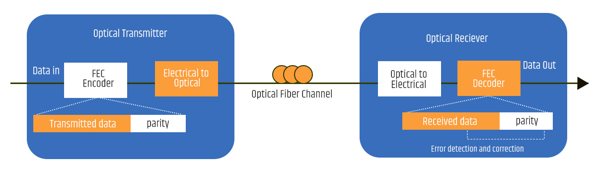
As you can see, to facilitate the development of optical technology-based interoperable transceivers across point-to-point networks, FEC definition is a necessary prerequisite.
Currently, industry trends are pushing for more open and disaggregated transport in high-volume, short-reach applications, while also removing proprietary elements and becoming interoperable.
Specifications
- Fully synchronous design using a single
- Clock
- Code Rate support of 1/2, 2/3, 3/4 and 5/6
- Block length of 648, 1256 and 1944
- Block length and code rate can be changed block by block at run time
- Number of Iterations from 10 to 18 or User-defined/Automatic
- Configurable soft input bit width
- Provides clock enable support at input and outputEasy-to-use interface with handshaking signals
- Supports all FPGA devices
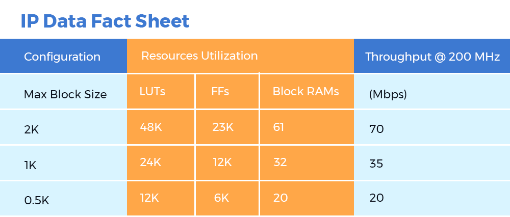
- The maximum synthesizable frequency is 200MHz
- More than 100 Mbps throughput at a block size of 1944
- Decoding algorithm: Offset Min-Sum
- Message Scheduling algorithm: Layered Belief Propagation (LBP)
Enhancement Available (On Demand)
- Support for different Code-Rates/Block-Sizes
- Support for different communication standards e.g. 802.11n, 802.11ac, 802.16e, etc
- System-Generator Model and Test-Bench availability (On demand)
Conclusion
Due to its exceptional performance and dependability in noisy conditions, LDPC codes have completely changed the field of digital communications error correction.
Their creation was a substantial breakthrough in coding theory since they combined practical efficacy with elegant mathematics.
The sparse matrix nature of LDPC codes makes them an effective tool for preserving data integrity in a variety of applications, such as satellite communications and wireless networks.
LDPC codes are still essential for overcoming noise problems and guaranteeing reliable information transfer as communication systems develop further.